If there were times you tried to organize documents with text, tables, and figures, I bet that you were bordering on the edge of frustration – at least, if you had been unlucky enough to not work on LaTeX.

So what is that? It is a free software to make all sort of documents – from reports to books. It is ever growing, with interfaces for easier use (for instance, Windows: MikTeX), and countless libraries (that is pieces of code to do things for you) and templates (already organized document).

What is extremely powerful with LaTeX, is that the entire document style can be changed by simple code lines (or by using a template or a library), it keeps tracks of anything you want to number (you just assign unique name to a table, chapter, figure… and LaTeX will assign a number depending on their position in the text and what you tell it is), you can site in the text/captions using pre-made bibliographies (i.e. BibTeX files can be created by Mendeley or JabRef ), you can use any alphabets (counting that you install the proper libraries), you can make beautiful equations (I do not joke, they are beautiful!), you can even by-pass software installation and create a document online (with ShareLaTex)… The versatility of LaTeX speaks for itself. The only time I do not use it by default is when I want to write a quick note or when I want to copy/paste some information from a webpage/pdf.

So why hesitating in taking the plunge? Well, first you need to accept that some code is employed to shape the document and that code is needed for specific cases – like making tables or equations.  It can be a tad overwhelming at first – mostly if you have none to bare knowledge and experience in programming softwares. But it is not that hard – mostly because of all the information available – on websites (officials ones, forums, fan-based ones), on all the countless pdf manuals and, of course, the help installed in the friendly user interface software (the ones which auto-suggest commands). The most difficult part is to understand how the templating works – and this can be understood much later since so many already made templates are not only built in the LaTeX software but also shared freely via libraries.

The first thing to do, in my opinion, is to install a user-friendly software (if you have up to little coding hours behind your back), or just the LaTeX basic interface (if you have confidence in your ability to grasp the coding logic of it). Then you should try to make the simplest of document style: an article.

It starts this way:

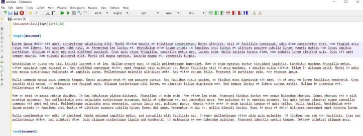
\documentclass[11pt]{article} \begin{document}

And end this way:

\end{document}

From here you can already see what I am about with auto-filling capacity of user-friendly software (like MikTeX): for each line of code that will start with a “\begin”, another need to be written down to signify to the software that it ends there with a “\end”. Next, you can notice that there are these dashes (“\”): they always (ALWAYS) indicates to the software that a piece of code – a command – start and need to be executed (that the software needs to do something specific). The command usually need to be specified, what to begin? What to do? Well, all depends on the type of libraries you use – but most libraries available built on the main software command (over wise the software sometimes just ignore it or refuse to compute – to finish producing a pdf document) – but all will be situated in the open/close curly braces (“{ }”). What about the first line of command? Well, this one is the core of the whole document. Without it, the program will not be able to run and produce an output. So what does it says? Well, we precise to the program what type of output document we want to create: they are in-built ones (for instance a book) and some that can be created by other users. Here it is an “article” type: this means that the document will not have a table of content or chapters (instead it will have sections) and that most likely it will be a good mix of text, tables, and figures. The open/close square brackets (“[ ]”) are used to give optional templating orders. Here we only set that the basic text (the one not formatted as a title) will be 11 points in font size. There are several options available (for instance to use single or double columns) and, again, libraries can be called upon to modify the templating further. But to be simple, just use this to start your document. 

To fill in text inside the document, you need to write (normally, apart for special characters like accentuated letters etc) within the “\begin” and “\end” commands. As a matter of fact, ALL things that you want to be in the document (that you want to appear in the document) should be within these boundaries – the rest (templating for instance) appears usually before the “\begin{document}” command. Just copy/paste random text in English from somewhere – LaTeX community loves Lorem Ipsum. At this point, it should look something like figure 1.

Next, it would be nice to compartmentalize the text into sections. Well, easy! Just use the command “\section{title}”. For this command, it is not necessary to have a “\begin” and “\end”, the “article” style as a built-in code to generate automatically numbered sections. They are numbered in the order in which they appear in the TeX document. Now, you can run (“compile” button on MikTeX) and compute (“build & view” button on MikTeX) (a bit different orders: “run” go through the code and tell you if everything works, while “compute” will give an output – if it is possible to).

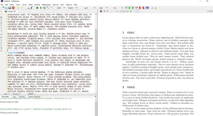
Now you might have something looking like figure 2. It would be good to add a title, date and author (at the very least) to the article right? Well, those belong to the templating parts – by design of the “article” style – and so the commands are built-in TeX and should be placed before the “\begin{document}” command.

The commands are very basics:

\title{text}
\date{text}
\author{names}

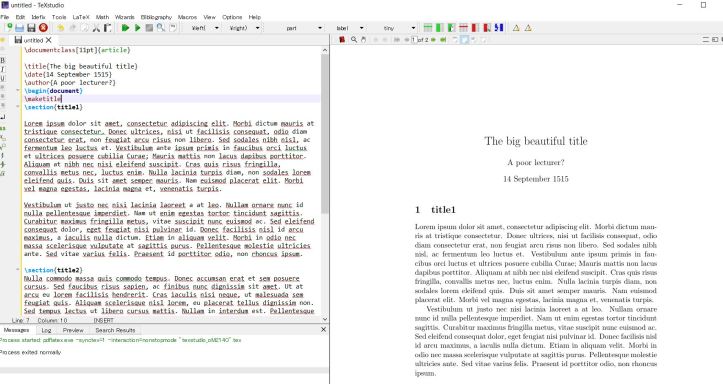
And to put the title (with all the other little information like date and such) in the document at the right place, you need to add one last command inside the “\begin{document}” – “\end{document}” area.

\maketitle

You have a lot of different options that can be used – for instance including a subtitle, using the date of today (the date you are compiling the output document), adding author’s addresses… Basically, if you want to do something just check on the “help” part of your software or search the web using keywords. For example, you want to add a logo near the title: “latex article add logo title” and usually you will manage to find either built-in commands or a new library to do what you want. If you do not find it, then you will have to adapt something existing (that do similar things) or completely change the type of document you produce. Now, you should have been able to produce an article in pdf format that resembles figure 3.

But what of the most interesting features of LaTeX? Well, for those, I would recommend installing libraries – they make things go much smoother and easier in the long run. To install libraries, you have to use basic commands (usual “install”-like ones) if you use the simple TeX software, overwise, the user-friendly ones have built-in menus to do so. Particularly, MikTeX has a whole different user interface to install packages of libraries – and to deal with the correct installation (to the proper folders).

To introduce figures in the document, I recommend using the package called “graphicx“, it always the best of figure manipulation within the document itself. For instance, you can set the figure to be of a certain percentage of the text size (of the column size), you can add labels (to keep track of it and cite it in the text), captions… You can import relatively any type of images (JPG, PNG, PDF, EPS…).

To be able to use the package (once installed) you will need to tell the TeX software to use it, by adding a command line just after the opening command (after “\documentclass[11pt]{article}”):

\usepackage{graphicx}

A basic command would look like that:

\begin{figure}[h]
\centering
\includegraphics[width=0.3\textwidth]{foldername/nameoffigure}
\caption{All the text you want}
\label{fig:nickname}
\end{figure}

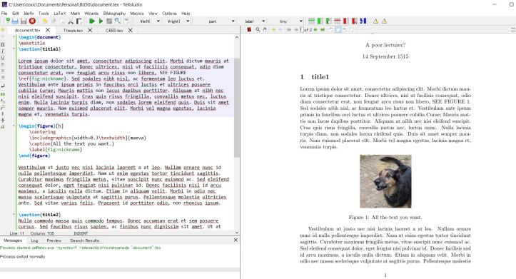
So what do we have here? Well, as expected, there are the “\begin” and “\end” command lines, this time delimiting within the document where the figure area is. The main command line that does most of the figure implementation is “\includegraphics”. As before, the options are in [ ] and the actual what (to include) is in { }. So how to import this figure into the document? First, save the tex document (it will be stored as a “.tex”) and take a figure and add it in the folder where the tex document is situated (then you do not need to have the name of the folder in { }, just the name of the figure) or in another folder created where you store the tex document. It is also possible to add figures stored on webpages using an URL, but this is something you will need to discover on your own (just search it online). What is the option specified in [ ]? It tells the software to take the figure original width and resize it to fit 30% of the text width (it goes from 0 to 1). What next? Well you notice that after the first command line “{figure}”, an option is used, here “[h]”. It is linked to how you want the figures to be placed in the document: do you want them all at the end? Or do you want the figure to be evenly distributed? The “h” means that the software should try to place it inline, so between the text where the figure command is placed. Then we have the command “\centering”, this one speak for itself: the figure will be centered within the document (it will adapt if you have a one or two-column type article). You can ask to be left/right align and much more. Esthetically, centering a figure is usually recommended – even more so for scientific papers. Finally, the graphicx package allows you to use command to implement a caption “\caption{}” and to label the figure “\label”. To be able to distinguished between different type of labels (if you want it so), you can specify which type of object this label is about. So {fig:} for a figure, {tab:} for a table, {eq:} for an equation… To be able to reference the figure in your document, just add the command:

\ref{fig:nickname}

where you want the figure to be cited. What is quite beautiful is that in an online pdf, the reference will be clickable: the reader can be transported to the cited figure directly!

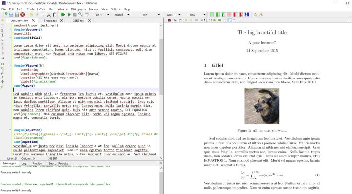
Now your article (and corresponding code) should look like figure 4.

There are myriad of options and templating possibilities, just familiarize yourself with tex first and then go for it (for instance, it is possible to make a small part -called “minipage” – to group several figures into one). It is also possible to draw on a figure or to simply create a figure with LaTeX – but this is not for beginners (I usually avoid it, as I prefer to create my figures using Inkscape).

Let’s make an equation now. I use the package “amsmath“, but several different ones exist. Just be careful of some compatibility problems that can arise between packages (some will compete for the formatting part of the document, messing it up). As for the figure package, the math pacakge need to be installed and then called in the document:

\documentclass[11pt]{article}
\usepackage{amsmath}

To create an equation, the simple command is:

\begin{equation}
\frac{2\alpha}{3\gamma} = \int_{- \infty}^{+ \infty} \cos(\pi) 2x^{2y} \times dx
\label{eq:nameeq}
\end{equation}

with the usual “\begin” and “\end” command and the specification of “{equation}” area. Then we can see different type of commands in-built in the library, such as “\frac” which gives a fraction, with the separating horizontal line set mid-level of regular text. The command “\alpha” is to obtain the greek letter alpha. The command “\int” gives an integral sign (with options of limits),  here with limits to infinity (“\infty”). You have also the command “\cos” which obsiouvly produced a cosinus symbol (the spacing of the letters composing “cos” will look different – you can try it by writing it too). Finally, the command “\times” displays one of the multiplication signs. Note that for the simple positive and negative signs, you can usually write them down without a command. For special equations and operations, you might want to use a specific command to produce the required sign. Of course, you can add a label (“\label”) which you can use to refer the equation in the text, using:

\ref{eq:nameeq}

Note that if you cite an equation/figure/table in a text before the object appears in the document (chronologically from top to bottom), you might need to compile the document several times (so that the TeX software is “aware” of the excistence of such object). If the software cannot find the cited object, an interogation symbol will appear where you referenced it. Figure 5 shows the resulting equation from the code above.

Finally, to insert a table in the document, I would use the package “tabularx“. Making a table – and making it stick and fit in the document – is the only aspect of LaTeX that is not so savy. But! But it is possible to produce a code using an online tool, using the webpage “tablegenerator“. Once you have installed and use the table package:

\documentclass[11pt]{article}
\usepackage{tabularx}

Go to the webpage and create a small table of 4 rows and 3 columns. You can decide to have lines separating the different raws/columns, you can change the text settings (right/centered/left align)… Just play with it as you see fit and copy the code generated. Then, it is easy to paste it in the document, add a label – and hop a numerated table that can be referenced in the text! In the “\begin{table}” – “\end{table}” area, you can use the usual commands like “\caption{}” and “\label{tab:}”. So that it can be used in the text, like this:

\ref{tab:nameoftable}

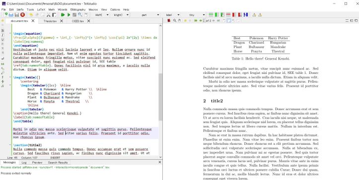
The final table in the document will look as depicted in figure 6. I added the command “\hline”, which produces a horizontal line and the command “\centering” to place the table in the middle of the text column. Esthetically, I find it more pleasing if a minimum amount of separation lines are drawn on a table. My final code is:

\begin{table}[]
\centering
\begin{tabular}{lcc} \hline
Best & Pokemon & Harry Potter \\ \hline
Dragon & Charizard & Hungarian \\
Plant & Bulbasaur & Mandrake \\
Horse & Ponyta & Thestral \\
\hline
\end{tabular}
\caption{Hello there! General Kenobi.}
\label{tab:nameoftable}
\end{table}

This is basically the most useful objects to manipulate in LaTeX.

Several other types of objects exists (like “\begin{itemize}”), but you should learn things steps by steps as the need for more complicated or strange objects arrises.

A small parting note: you can use equation-like command if you set yourself in the math environment by using dollar signs (“$  $”). The math environment make the letters look different than the main text, so use it mostly for the specific symbol or mathematical notations you want to make. For exemple you can write a chemical formula this way:

I write normal text but then I want to write the formula of water then I write on my latex file H$_2$O, so that the 2 appears as underscore of H.

I would also make you take note of the fact that it is possible to nestle tex files within tex files, this is particularly useful for writing long documents such as books, where each chapter or section is a separate tex file (that you cannot compute on its own, since you will just write as if you where writing between the “\begin{document}” and “\end{document}”. The command is usually something like “ \input{filename}”.

That is all folks! I hope I gave you the basics to start playing with TeX ~ enjoy your beautifully tailored books, articles, beamers, CVs and more ^^.